Artificial Neural Networks: Mathematics of Backpropagation (Part 4)

Up until now, we haven't utilized any of the expressive non-linear power of neural networks - all of our simple one layer models corresponded to a linear model such as multinomial logistic regression. These one-layer models had a simple derivative. We only had one set of weights the fed directly to our output, and it was easy to compute the derivative with respect to these weights. However, what happens when we want to use a deeper model? What happens when we start stacking layers? 

No longer is there a linear relation in between a change in the weights and a change of the target. Any perturbation at a particular layer will be further transformed in successive layers. So, then, how do we compute the gradient for all weights in our network? This is  where we use the backpropagation algorithm.

Backpropagation, at its core, simply consists of repeatedly applying the chain rule through all of the possible paths in our network. However, there are an exponential number of directed paths from the input to the output. Backpropagation's real power arises in the form of a dynamic programming algorithm, where we reuse intermediate results to calculate the gradient. We transmit intermediate errors backwards through a network, thus leading to the name backpropagation. In fact, backpropagation is closely related to forward propagation, but instead of propagating the inputs forward through the network, we propagate the error backwards.

Most explanations of backpropagation start directly with a general theoretical derivation, but I’ve found that computing the gradients by hand naturally leads to the backpropagation algorithm itself, and that’s what I’ll be doing in this blog post. This is a lengthy section, but I feel that this is the best way to learn how backpropagation works.

I’ll start with a simple one-path network, and then move on to a network with multiple units per layer. Finally, I’ll derive the general backpropagation algorithm. Code for the backpropagation algorithm will be included in my next installment, where I derive the matrix form of the algorithm.

Examples: Deriving the base rules of backpropagation

Remember that our ultimate goal in training a neural network is to find the gradient of each weight with respect to the output: $$\begin{align} \frac{\partial E}{\partial w_{i\rightarrow j}} \end{align}$$ We do this so that we can update the weights incrementally using stochastic gradient descent: $$\begin{align*} w_{i\rightarrow j} =& w_{i\rightarrow j} -\eta \frac{\partial E}{\partial w_{i\rightarrow j}} \end{align*}$$

For a single unit in a general network, we can have several cases: the unit may have only one input and one output (case 1), the unit may have multiple inputs (case 2), or the unit may have multiple outputs (case 3). Technically there is a fourth case: a unit may have multiple inputs and outputs. But as we will see, the multiple input case and the multiple output case are independent, and we can simply combine the rules we learn for case 2 and case 3 for this case.

I will go over each of this cases in turn with relatively simple multilayer networks, and along the way will derive some general rules for backpropagation.  At the end, we can combine all of these rules into a single grand unified backpropagation algorithm for arbitrary networks.

Case 1: Single input and single output

Suppose we have the following network:

A simple "one path" network.

We can explicitly write out the values of each of variable in this network: $$ \begin{align} s_j =&\ w_1\cdot x_i\\ z_j =&\ \sigma(in_j) = \sigma(w_1\cdot x_i)\\ s_k =&\ w_2\cdot z_j\\ z_k =&\ \sigma(in_k) = \sigma(w_2\cdot\sigma(w_1\cdot x_i))\\ s_o =&\ w_3\cdot z_k\\ \hat{y}_i =&\ in_o = w_3\cdot\sigma(w_2\cdot\sigma(w_1\cdot x_i))\\ E =&\ \frac{1}{2}(\hat{y}_i - y_i)^2 = \frac{1}{2}(w_3\cdot\sigma(w_2\cdot\sigma(w_1\cdot x_i)) - y_i)^2 \end{align} $$ For this simple example, it's easy to find all of the derivatives by hand. In fact, let's do that now. I am going to color code certain parts of the derivation, and see if you can deduce a pattern that we might exploit in an iterative algorithm. First, let's find the derivative for $w_{k\rightarrow o}$ (remember that $\hat{y} = w_{k\rightarrow o}z_k$, as our output is a linear unit): $$ \begin{align} \frac{\partial E}{\partial w_{k\rightarrow o}} =&\ \frac{\partial}{\partial w_{k\rightarrow o}} \frac{1}{2}(\hat{y}_i - y_i)^2\\ =&\ \frac{\partial}{\partial w_{k\rightarrow o}} \frac{1}{2}(w_{k\rightarrow o}\cdot z_k - y_i)^2\\ =&\ (w_{k\rightarrow o}\cdot z_k - y_i)\frac{\partial}{\partial w_{k\rightarrow o}}(w_{k\rightarrow o}\cdot z_k - y_i)\\ =&\ \color{blue}{(\hat{y_i} - y_i)}(z_k) \end{align} $$ Finding the weight update for $w_{i\rightarrow k}$ is also relatively simple: $$ \begin{align} \frac{\partial E}{\partial w_{j\rightarrow k}} =&\ \frac{\partial}{\partial w_{j\rightarrow k}} \frac{1}{2}(\hat{y}_i - y_i)^2\\ =&\ (\hat{y}_i-y_i)\left( \frac{\partial}{\partial w_{j\rightarrow k}} (w_{k\rightarrow o}\cdot\sigma(w_{j\rightarrow k}\cdot z_j) - y_i) \right)\\ =&\ (\hat{y}_i-y_i)(w_{k\rightarrow o})\left( \frac{\partial}{\partial w_{j\rightarrow k}} \sigma(w_{j\rightarrow k}\cdot z_j) \right)\\ =&\ (\hat{y}_i-y_i)(w_{k\rightarrow o})\left( \sigma(s_k)(1-\sigma(s_k)) \frac{\partial }{\partial w_{j\rightarrow k}}(w_{j\rightarrow k}\cdot z_j) \right)\\ =&\ \color{blue}{(\hat{y}_i-y_i)}\color{red}{(w_{k\rightarrow o})\left( \sigma(s_k)(1-\sigma(s_k)\right)}(z_j) \end{align} $$ Again, finding the weight update for $w_{i\rightarrow j}$ consists of some straightforward calculus: $$ \begin{align} \frac{\partial E}{\partial w_{i\rightarrow j}} =&\ \frac{\partial}{\partial w_{i\rightarrow j}} \frac{1}{2}(\hat{y}_i-y_i)^2\\ =&\ (\hat{y}_i-y_i)\left( \frac{\partial}{\partial w_{i\rightarrow j}} (\hat{y}_i-y_i) \right)\\ =&\ (\hat{y}_i-y_i)(w_{k\rightarrow o})\left( \frac{\partial}{\partial w_{i\rightarrow j}}\cdot\sigma(w_{j\rightarrow k}\cdot\sigma(w_{i\rightarrow j}\cdot x_i))\right)\\ =&\ (\hat{y}_i-y_i)(w_{k\rightarrow o})(\sigma(s_k)(1-\sigma(s_k)))(w_{j\rightarrow k})\left( \frac{\partial}{\partial w_{i\rightarrow j}}\sigma(w_{i\rightarrow j}\cdot x_i) \right)\\ =&\ \color{blue}{(\hat{y}_i-y_i)}\color{red}{(w_{k\rightarrow o})(\sigma(s_k)(1-\sigma(s_k)))}\color{OliveGreen}{(w_{j\rightarrow k})(\sigma(s_j)(1-\sigma(s_j)))}(x_i) \end{align} $$
By now, you should be seeing a pattern emerging, a pattern that hopefully we could encode with backpropagation. We are reusing multiple values as we compute the updates for weights that appear earlier and earlier in the network. Specifically, we see the derivative of the network error, the weighted derivative of unit $k$'s output with respect to $s_k$, and the weighted derivative of unit $j$'s output with respect to $s_j$.
So, in summary, for this simple network, we have: $$ \begin{align} \Delta w_{i\rightarrow j} =&\ -\eta\left[ \color{blue}{(\hat{y}_i-y_i)}\color{red}{(w_{k\rightarrow o})(\sigma(s_k)(1-\sigma(s_k)))}\color{OliveGreen}{(w_{j\rightarrow k})(\sigma(s_j)(1-\sigma(s_j)))}(x_i) \right]\\ \Delta w_{j\rightarrow k} =&\ -\eta\left[ \color{blue}{(\hat{y}_i-y_i)}\color{red}{(w_{k\rightarrow o})\left( \sigma(s_k)(1-\sigma(s_k)\right)}(z_j)\right]\\ \Delta w_{k\rightarrow o} =&\ -\eta\left[ \color{blue}{(\hat{y_i} - y_i)}(z_k)\right] \end{align} $$

Case 2: Handling multiple inputs

Consider the more complicated network, where a unit may have more than one input:

What happens to a weight when it leads to a unit that has multiple inputs? Is $w_{i\rightarrow k}$'s update rule affected by $w_{j\rightarrow k}$'s update rule? To see, let's derive the update for $w_{i\rightarrow k}$ by hand: $$ \begin{align} \frac{\partial E}{w_{i\rightarrow k}} =& \frac{\partial}{w_{i\rightarrow k}}\frac{1}{2}(\hat{y}_i - y_i)^2\\ =&\ (\hat{y}_i - y_i)\left( \frac{\partial}{w_{i\rightarrow k}}z_k w_{k\rightarrow o} \right)\\ =&\ (\hat{y}_i - y_i)(w_{k\rightarrow o})\left( \frac{\partial}{w_{i\rightarrow k}}\sigma\left( s_k \right) \right)\\ =&\ (\hat{y}_i - y_i)(\sigma(s_k)(1-\sigma(s_k)) w_{k\rightarrow o})\left( \frac{\partial}{w_{i\rightarrow k}}\left( z_iw_{i\rightarrow k} + z_jw_{j\rightarrow k} \right) \right)\\ =&\ (\hat{y}_i - y_i)(\sigma(s_k)(1-\sigma(s_k)) w_{k\rightarrow o})z_i \end{align} $$
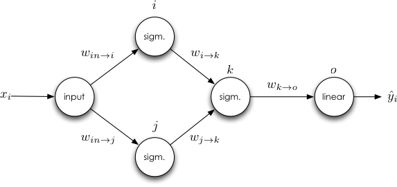
Here we see that the update for $w_{i\rightarrow k}$ does not depend on $w_{j\rightarrow k}$'s derivative, leading to our first rule: The derivative for a weight is not dependent on the derivatives of any of the other weights in the same layer. Thus we can update weights in the same layer in isolation. There is a natural ordering of the updates - they only depend on the values of other weights in the same layer, and (as we shall see), the derivatives of weights further in the network. This ordering is good news for the backpropagation algorithm.

Case 3: Handling multiple outputs

Now let's examine the case where a hidden unit has more than one output.

Based on the previous sections, the only "new" type of weight update is the derivative of $w_{in\rightarrow j}$. The difference in the multiple output case is that unit $i$ has more than one immediate successor, so (spoiler!) we must sum the error accumulated along all paths that are rooted at unit $i$. Let's explicitly derive the weight update for $w_{in\rightarrow i}$ (to keep track of what's going on, we define $\sigma_i(\cdot)$ as the activation function for unit $i$): $$ \begin{align} \frac{\partial E}{w_{in\rightarrow i}} =& \frac{\partial}{w_{in\rightarrow i}}\frac{1}{2}(\hat{y}_i - y_i)^2\\ =&\ (\hat{y}_i - y_i)\left( \frac{\partial}{w_{in\rightarrow i}}(z_j w_{j\rightarrow o} + z_k w_{k\rightarrow o}) \right)\\ =&\ (\hat{y}_i - y_i)\left( \frac{\partial}{w_{in\rightarrow i}}(\sigma_j(s_j) w_{j\rightarrow o} + \sigma_k(s_k)w_{k\rightarrow o}) \right)\\ =&\ (\hat{y}_i - y_i)\left( w_{j\rightarrow o}\sigma_j'(s_j) \frac{\partial}{w_{in\rightarrow i}}s_j + w_{k\rightarrow o}\sigma_k'(s_k) \frac{\partial}{w_{in\rightarrow i}}s_k \right)\\ =&\ (\hat{y}_i - y_i)\left( w_{j\rightarrow o}\sigma_j'(s_j) \frac{\partial}{w_{in\rightarrow i}}z_iw_{i\rightarrow j} + w_{k\rightarrow o}\sigma_k'(s_k) \frac{\partial}{w_{in\rightarrow i}}z_iw_{i\rightarrow k} \right)\\ =&\ (\hat{y}_i - y_i)\left( w_{j\rightarrow o}\sigma_j'(s_j) \frac{\partial}{w_{in\rightarrow i}}\sigma_i(s_i)w_{i\rightarrow j} + w_{k\rightarrow o}\sigma_k'(s_k) \frac{\partial}{w_{in\rightarrow i}}\sigma_i(s_i)w_{i\rightarrow k} \right)\\ =&\ (\hat{y}_i - y_i)\left( w_{j\rightarrow o}\sigma_j'(s_j) w_{i\rightarrow j}\sigma'_i(s_i)\frac{\partial}{w_{in\rightarrow i}}s_i + w_{k\rightarrow o}\sigma_k'(s_k) w_{i\rightarrow k}\sigma'_i(s_i) \frac{\partial}{w_{in\rightarrow i}}s_i \right)\\ =&\ (\hat{y}_i - y_i)\left( w_{j\rightarrow o}\sigma_j'(s_j) w_{i\rightarrow j}\sigma'_i(s_i) + w_{k\rightarrow o}\sigma_k'(s_k) w_{i\rightarrow k}\sigma'_i(s_i) \right)x_i \end{align} $$
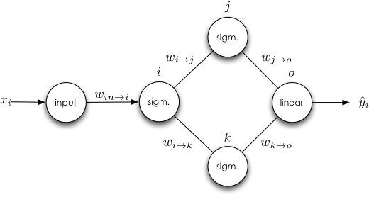
There are two things to note here. The first, and most relevant, is our second derived rule: the weight update for a weight leading to a unit with multiple outputs is dependent on derivatives that reside on both paths.

But more generally, and more importantly, we begin to see the relation between backpropagation and forward propagation. During backpropagation, we compute the error of the output. We then pass the error backward and weight it along each edge. When we come to a unit, we multiply the weighted backpropagated error by the unit's derivative. We then continue backpropagating this error in the same fashion, all the way to the input. Backpropagation, much like forward propagation, is a recursive algorithm. In the next section, I introduce the notion of an error signal, which allows us to rewrite our weight updates in a compact form.

Error Signals

Deriving all of the weight updates by hand is intractable, especially if we have hundreds of units and many layers. But we saw a pattern emerge in the last few sections - the error is propagated backwards through the network. In this section, we define the error signal, which is simply the accumulated error at each unit. For now, let's just consider the contribution of a single training instance (so we use $\hat{y}$ instead of $\hat{y}_i$).

We define the recursive error signal at unit $j$ as: $$ \begin{align} \delta_j =&\ \frac{\partial E}{\partial s_j} \end{align} $$ In layman's terms, it is a measure of how much the network error varies with the input to unit $j$. Using the error signal has some nice properties - namely, we can rewrite backpropagation in a more compact form. To see this, let's expand $\delta_j$: $$ \begin{align} \delta_j =&\ \frac{\partial E}{\partial s_j}\\ =&\ \frac{\partial}{\partial s_j}\frac{1}{2}(\hat{y} - y)^2\\ =&\ (\hat{y} - y)\frac{\partial \hat{y}}{\partial s_j} \end{align} $$ Consider the case where unit $j$ is an output node. This means that $\hat{y} = f_j(s_j)$ (if unit $j$'s activation function is $f_j(\cdot)$), so $\frac{\partial \hat{y}}{\partial s_j}$ is simply $f_j'(s_j)$, giving us $\delta_j = (\hat{y} - y)f'_j(s_j)$.

Otherwise, unit $j$ is a hidden node that leads to another layer of nodes $k\in \text{outs}(j)$. We can expand $\frac{\partial \hat{y}}{\partial s_j}$ further, using the chain rule: $$ \begin{align} \frac{\partial \hat{y}}{\partial s_j} =&\ \frac{\partial \hat{y}}{\partial z_j}\frac{\partial z_j}{\partial s_j}\\ =&\ \frac{\partial \hat{y}}{\partial z_j}f_j'(s_j) \end{align} $$ Take note of the term $\frac{\partial \hat{y}}{\partial z_j}$. Multiple units depend on $z_j$, specifically, all of the units $k\in\text{outs}(j)$. We saw in the section on multiple outputs that a weight that leads to a unit with multiple outputs does have an effect on those output units. But for each unit $k$, we have $s_k = z_jw_{j\rightarrow k}$, with each $s_k$ not depending on any other $s_k$. Therefore, we can use the chain rule again and sum over the output nodes $k\in\text{outs}(j)$: $$ \begin{align} \frac{\partial \hat{y}}{\partial s_j} =&\ f_j'(s_j)\sum_{k\in\text{outs}(j)} \frac{\partial \hat{y}}{\partial s_k}\frac{\partial s_k}{\partial z_j}\\ =&\ f_j'(s_j)\sum_{k\in\text{outs}(j)} \frac{\partial \hat{y}}{\partial s_k}w_{j\rightarrow k} \end{align} $$ Plugging this equation back into the function $\delta_j = (\hat{y} - y) \frac{\partial \hat{y}}{\partial s_j}$, we get: $$ \begin{align} \delta_j =& (\hat{y} - y)f_j'(s_j)\sum_{k\in\text{outs}(j)} \frac{\partial \hat{y}}{\partial s_k}w_{j\rightarrow k} \end{align} $$ Based on our definition of the error signal, we know that $\delta_k = (\hat{y} - y) \frac{\partial \hat{y}}{\partial s_k}$, so if we push $(\hat{y} - y)$ into the summation, we get the following recursive relation: $$ \begin{align} \delta_j =& f_j'(s_j)\sum_{k\in\text{outs}(j)} \delta_k w_{j\rightarrow k} \end{align} $$ We now have a compact representation of the backpropagated error. The last thing to do is tie everything together with a general algorithm.

The general form of backpropagation

Recall the simple network from the first section:

We can use the definition of $\delta_i$ to derive the values of all the error signals in the network: $$ \begin{align} \delta_o =&\ (\hat{y} - y) \text{ (The derivative of a linear function is 1)}\\ \delta_k =&\ \delta_o w_{k\rightarrow o}\sigma(s_k)(1 - \sigma(s_k))\\ \delta_j =&\ \delta_k w_{j\rightarrow k}\sigma(s_j)(1 - \sigma(s_j)) \end{align} $$ Also remember that the explicit weight updates for this network were of the form: $$ \begin{align} \Delta w_{i\rightarrow j} =&\ -\eta\left[ \color{blue}{(\hat{y}_i-y_i)}\color{red}{(w_{k\rightarrow o})(\sigma(s_k)(1-\sigma(s_k)))}\color{OliveGreen}{(w_{j\rightarrow k})(\sigma(s_j)(1-\sigma(s_j)))}(x_i) \right]\\ \Delta w_{j\rightarrow k} =&\ -\eta\left[ \color{blue}{(\hat{y}_i-y_i)}\color{red}{(w_{k\rightarrow o})\left( \sigma(s_k)(1-\sigma(s_k)\right)}(z_j)\right]\\ \Delta w_{k\rightarrow o} =&\ -\eta\left[ \color{blue}{(\hat{y_i} - y_i)}(z_k)\right] \end{align} $$ By substituting each of the error signals, we get: $$ \begin{align} \Delta w_{k\rightarrow o} =&\ -\eta \delta_o z_k\\ \Delta w_{j\rightarrow k} =&\ -\eta \delta_kz_j\\ \Delta w_{i\rightarrow j} =&\ -\eta \delta_jx_i \end{align} $$ As another example, let's look at the more complicated network from the section on handling multiple outputs:

We can again derive all of the error signals: $$ \begin{align} \delta_o =&\ (\hat{y} - y)\\ \delta_k =&\ \delta_o w_{k\rightarrow o}\sigma(s_k)(1 - \sigma(s_k))\\ \delta_j =&\ \delta_o w_{j\rightarrow o}\sigma(s_j)(1 - \sigma(s_j))\\ \delta_i =&\ \sigma(s_i)(1 - \sigma(s_i))\sum_{k\in\text{outs}(i)}\delta_k w_{i\rightarrow k} \end{align} $$ Although we did not derive all of these weight updates by hand, by using the error signals, the weight updates become (and you can check this by hand, if you'd like): $$ \begin{align} \Delta w_{k\rightarrow o} =&\ -\eta \delta_o z_k\\ \Delta w_{j\rightarrow o} =&\ -\eta \delta_o z_j\\ \Delta w_{i\rightarrow k} =&\ -\eta \delta_k z_i\\ \Delta w_{i\rightarrow j} =&\ -\eta \delta_j z_i\\ \Delta w_{in\rightarrow i} =&\ -\eta \delta_i x_i \end{align} $$ It should be clear by now that we've derived a general form of the weight updates, which is simply $\Delta w_{i\rightarrow j} = -\eta \delta_j z_i$.

The last thing to consider is the case where we use a minibatch of instances to compute the gradient. Because we treat each $y_i$ as independent, we sum over all training instances to compute the full update for a weight (we typically scale by the minibatch size $N$ so that steps are not sensitive to the magnitude of $N$). For each separate training instance $y_i$, we add a superscript $(y_i)$ to the values that change for each training example: $$ \begin{align} \Delta w_{i\rightarrow j} =&\ -\frac{\eta}{N} \sum_{y_i} \delta_j^{(y_i)}z_i^{(y_i)} \end{align} $$ Thus, the general form of the backpropagation algorithm for updating the weights consists the following steps:

1. Feed the training instances forward through the network, and record each $s_j^{(y_i)}$ and $z_{j}^{(y_i)}$.
2. Calculate the error signal $\delta_j^{(y_i)}$ for all units $j$ and each training example $y_{i}$. If $j$ is an output node, then $\delta_j^{(y_i)} = f'_j(s_j^{(y_i)})(\hat{y}_i - y_i)$. If $j$ is not an output node, then $\delta_j^{(y_i)} = f'_j(s_j^{(y_i)})\sum_{k\in\text{outs}(j)}\delta_k^{(y_i)} w_{j\rightarrow k}$.
3. Update the weights with the rule $\Delta w_{i\rightarrow j} =-\frac{\eta}{N} \sum_{y_i} \delta_j^{(y_i)}z_i^{(y_i)}$.

Conclusions

Hopefully you've gained a full understanding of the backpropagation algorithm with this derivation. Although we've fully derived the general backpropagation algorithm in this chapter, it's still not in a form amenable to programming or scaling up. In the next post, I will go over the matrix form of backpropagation, along with a working example that trains a basic neural network on MNIST.